State of the Art

When characterizing a propellant, one of the most critical aspects is to find the linear burn rate of the propellant as a function of pressure. This, along with c-star, allows one to model the internal ballistics of a given motor. The standard for burn rate characterization is done with strand burner apparatuses. These devices are essentially a pressure vessel which are regulated to a certain pressure. A strand of solid propellant with its outer surface inhibited except for the strand end is then placed in the pressure vessel. The end of the strand can then be ignited and the burn rate observed either through optical means, or by placing thin nichrome wires within the strand which melt as the burn progresses, and continuity across the wire is measured. Making a strand burner apparatus with sufficient volume or pressure regulation capabilities to enable constant pressure, as well as making the pneumatic systems for pressurization, gas storage, and fail safes make the system complexity considerable.

Computing Burn Rate from Static Motor Test

Although less accurate, one can also compute estimated burn rate versus pressure by static firing a solid motor if there is pressure data and the grain geometry is known. This is the case in our test apparatus. This method revolves around the characteristic velocity value, which is computed after every burn for that specific burn. It is assumed to be constant over the entire burn. The experimental equation for characteristic velocity, represented by \(c^*\) is:

$$c^* = \frac{P_{0} * A_{t} }{\dot{m}}$$

where \(P_{0}\) is chamber pressure, \(A_{t}\) is throat area, and \(\dot{m}\) is mass flow rate. If motor operation is assumed as steady state (only true for a certain region of burn), mass flow rate can be substituted with \(\dot{m} = r * A_{b} * \rho\), where \(r\) is burnrate, \(A_{b}\) is burning surface area, and \(\rho\) is grain density. Combining these 2 equations yields:

\[r = \frac{P_{0}*A_{t}}{\rho * A_{b} * c^*}\]

In this equation, burn rate is what is being computed. Throat area, c-star, and propellant density are assumed constant and either known, or computed beforehand. At each instant there is a chamber pressure measurement. This leaves only burning surface as the only remaining value to be computed. This is known initially. So one can compute the burn rate initially, then use that burn rate, grain geometry, and time step to get the next burning surface area. This process is done by taking the original dimensions of the grain, then recomputing new dimensions based on linear burn distance. Linear burn distance is computed by \(d = r*\Delta t\). For a BATES grain, this distance is the decrease in web thickness, and half the decrease in grain length. This process gives the burning surface area, and thus burn rate for each point. Finally, the burn rate values can be graphed against their pressure values at each point.

Although theoretically sound, this method assumes steady state burning for the duration of the burn. The burn is not steady state during the start and stop transients. Because of this, the method outlined in the paragraph before will not yield the correct result (the entire grain would be computed as being burned through before the end of data is gotten to, or there would still be grain left when at end of data). The above method must be modified to only be applied during steady state operation. Only analyzing data in the steady state region makes it so the initial burning surface area is not known directly since some of the grain has burnedaway during the startup transient. To determine the burning area at the beginning of steady state, the program “guesses” at different initial burned web thicknesses. It attempts to find the initial burn distance so that there is no final web thickness computed at the end of steady state operation, i.e. all of the grain is burned away at the end of the burn.

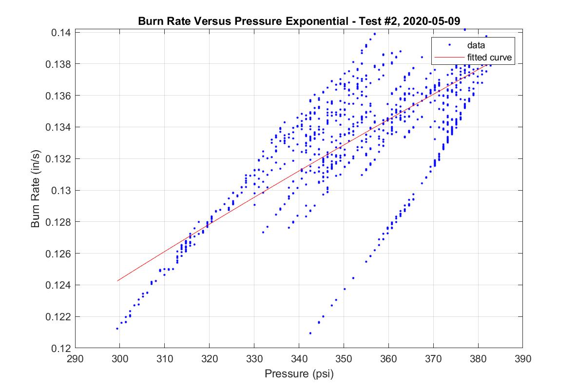
Results

Using the method above burn rate can then be related to pressure by setting pressure as the independent variable for each time point and graphing the computed burn rate. A regression can then be done to yield a curve in the form \(r = a * {P_{0}}^n\) which serves as a characterization of burn rate versus pressure over a given pressure range. A sample burn rate computation from one a test is shown below. The equation of fit for this data is \(r = 0.0107 * {P_{0}}^{0.429}\), with burn rate in in/s, and pressure in psi. It can be seen that the burn rate points do not line up exactly. This is because the burn rate is computed as higher in the beginning of the burn when pressure is increasing, versus at the end of the burn when pressure is decreasing. This is most likely due to uneven burning geometry